Weight Standardization: A new normalization in town

Recently a new normalization technique is proposed not for the activations but for the weights themselves in the paper Weight Standardization.

In short, to get new state of the art results, they combined Batch Normalization and Weight Standardization. So in this post, I discuss what is weight standardization and how it helps in the training process, and I will show my own experiments on CIFAR-10 which you can also follow along.

Fig1; Taken from the paper. Shows a clear comparison of all normalizations.

The notebook for the post is at this link. For my experiments, I will use cyclic learning. As the paper discusses training with constant learning rates, I would use cyclic LR as presented by Leslie N. Smith in his report. I am working on making a post on state-of-the methods for training neural networks in 2019 where I would summarize all these methods along with the ones that I learned from fastai courses.

To make things cleaner I would use this notation:-

1. BN -> Batch Normalization
2. GN -> Group Normalization
3. WS -> Weight Standardization

What is wrong with BN and GN?

Ideally, nothing is wrong with them. But to get the most benefit out of BN we have to use a large batch size. And when we have smaller batch sizes we prefer to use GN. (By smaller I mean 1–2 images/GPU).

Why is this so?

To understand it we have to see how BN works. To make things simple, consider we have only one-channel on which we want to apply BN and we have 2 images as our batch size.

Now we would compute the mean and variance using the 2 images and then normalize the one-channel of the 2 images. So we used 2 images to compute mean and variance. This is the problem.

By increasing batch size, we are able to sample the value of mean and variance from a larger population, which means that the computed mean and variance would be closer to their real values.

GN was introduced for cases of small batch sizes but it was not able to meet the results that BN was able to achieve using larger batch sizes.

How these normalizations actually help?

It is one of the leading areas of research. But it was recently shown in the paper Fixup Initialization: Residual Learning without Normalization the reason for the performance gains using BN.

In short, it helps make the loss surface smooth.

Fig1: Remember when we train NNs we are in millions of dimensions. Here I show an example of loss varying with only one parameter.

When we make the loss surface smooth we can take longer steps, which means we can increase our learning rate. So using Batch Norm actually stabilizes our training and also makes it faster.

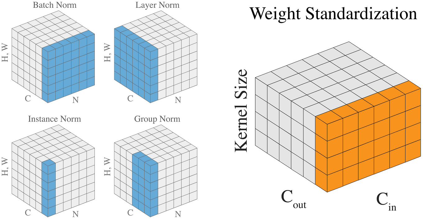
Weight Standardization

Unlike BN and GN that we apply on activations i.e the output of the conv layer, we apply Weight Standardization on the weights of the conv layer itself. So we are applying WS to the kernels that our conv layer uses.

How does this help?

For the theoretical justification see the original paper where they prove WS reduces the Lipschitz constants of the loss and the gradients.

But there are easier ways to understand it.

First, consider the optimizer we use. The role of the optimizer is to optimize the weights of our model, but when we apply normalization layers like BN, we do not normalize our weights, but instead, we normalize the activations which are optimizer does not even care about.

By using WS we are essentially normalizing the gradients during the backpropagation.

The authors of the paper tested WS on various computer vision tasks and they were able to achieve better results with the combination of WS+GN and WS+BN. The tasks that they tested on included:

1. Image Classification
2. Object Detection
3. Video Recognition
4. Semantic Segmentation
5. Point Cloud Classification

Enough talk, let’s go to experiments

The code is available in the notebook.

How to implement WS?

class Conv2d(nn.Module):
    def __init__(self, in_chan, out_chan, kernel_size, stride=1, 
                 padding=0, dilation=1, groups=1, bias=True):
        super().__init__(in_chan, out_chan, kernel_size, stride, 
                         padding, dilation, groups, bias)
def forward(self, x):
        weight = self.weight
        weight_mean = weight.mean(dim=1, keepdim=True).mean(dim=2,
                                  keepdim=True).mean(dim=3, keepdim=True)
        weight = weight - weight_mean
        std = weight.view(weight.size(0), -1).std(dim=1).view(-1,1,1,1)+1e-5
        weight = weight / std.expand_as(weight)
        return F.conv2d(x, weight, self.bias, self.stride,
                        self.padding, self.dilation, self.groups)

First, let’s try out at batch size = 64

This will provide a baseline of what we should expect. For this, I create 2 resnet18 models:

1. resnet18 -> It uses the nn.Conv2d layers
2. resnet18_ws -> It uses above Conv2d layer which uses weight standardization

I change the head of resnet model, as CIFAR images are already 32 in size and I don’t want to half their size initially. The code can be found in the notebook. And for the CIFAR dataset, I use the official train and valid split.

First I plot the value of loss v/s learning rate. For the theory behind it, refer to fastai courses or Leslie N. Smith’s papers.

For those not familiar with loss v/s learning_rate graph. We are looking for the maximum value of lr at which the loss value starts increasing.

In this case the max_lr is around 0.0005. So let’s try to train model for some steps and see. In case you wonder in the second case the graph is flatter around 1e-2, it is because the scale of the two graphs is different.

So now let’s train our model and see what happens. I am using the fit_one_cycle to train my model.

There is not much difference between the two as valid loss almost remains the same.

So not, let’s test it out for small batches. So now I take a batch size of 2 and train the models in a similar manner.

One thing that I should add here, is the loss diverged quickly when I used only BN, after around 40 iterations, while in the case of WS+BN the loss did not diverge.

There is not much difference in the loss values, but the time to run each cycle increased very much.

Also, I run some more experiments where I used a batch size of 256. Although, I could use a larger learning rate but the time taken to complete the cycle increased. The results are shown below

Again, in the graph we see we can use a larger learning rate.

From the above experiments, I think I would prefer not to use Weight Standardization when I am using cyclic learning. For large batch sizes, it even gave worse performance and for smaller batch sizes, it gave almost similar results, but using weight standardization we added a lot of time to our computation, which we could have used to train our model with Batch Norm alone.

For constant learning rate, I think weight standardization still makes sense as there we do not change our learning rate in the training process, so we must benefit from the smoother loss function. But in the case of cyclic learning, it does not offer us a benefit.